Decision Tree Regressors
Most people practicing data science would be aware of tree based learning methods like XGBoost. Despite LLMs occupying the current spotlight, these tree based methods are still widely used and even outperform neural networks when dealing with tabular/structured data.
Neural networks, while powerful in their own right, excel at modelling unstructured data through their architecture, be it positional encoding + self-attention for seq2seq models or convolutions for images. Tabular data still forms a large part of most companies’ data source and building models that leverage such data can yield great value through recommendation systems and targeted marketing campaigns.
I have always been interested in learning about the inner workings of such tree based methods, and will explain them in detail, starting with the decision tree regressor which is the foundation for tree based methods. While learning and writing on this topic I came across and was inspired by a useful blog that helped me gain an intuitive understanding on these methods.
Before diving in to decision tree regressors, what is a regressor? A regressor is a trained model that learns a function which returns or outputs a continuous variable based on a given input. For example, a regressor can learn a simple linear function y = 2x. Inputting a value of 5 to this regressor would yield a value of 10 as the target output.
Overview
How do we estimate a function? Given a set of training data inputs X and label y we can assign mean(y) for any value of X.
\[f(x) = mean(y)\]We can extend this further to apply thresholds at certain values of \(x\) where
\[f(x<n) = mean(y\mid x <n)\]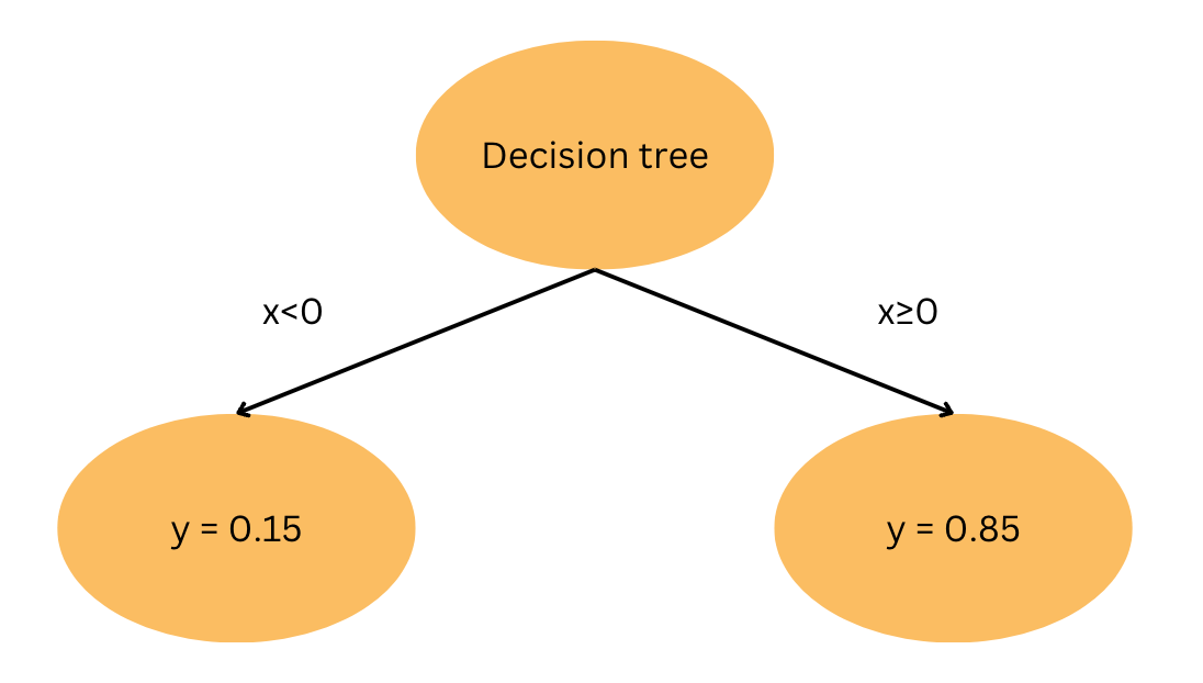
This can also be illustrated with the binary tree above, where the threshold n=0. If \(x\) is less than 0, the model predicts y=0.15 and it predicts y=0.85 for any value greater or equal to 0. The binary tree above shows one threshold value with depth=1. We can illustrate this example more clearly when fitting a decision tree regressor of various depths to a sigmoid function: \(y = \frac{1}{1 + e^{-x}}\).
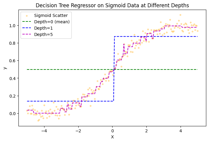
From the image above we can see how well our decision tree regressor fits the sigmoid function at various depths of the tree. Depth=0 is denoted by the green line where we naively assume that any value x will approximate the mean of y. For depth=1 we can see a threshold at \(x=0\) and gradually see our model increasingly fit the sigmoid function with increasing depth.
Code Explained
def mean(x):
    return sum(x) / len(x) if x else 0.0

def variance(x):
    if len(x) > 1:
        return sum((i - mean(x)) ** 2 for i in x) / len(x)
    return 0.0
Before going through the decision tree regressor line by line we first define two helper functions to obtain the mean and variance. Mean is used to determine the approximate value at each threshold, while variance (also known as mean square error) determines which threshold we use.
root = {}
stack = [{"X": X, "y": y, "depth": 0, "node": root}]

current = stack.pop()
Xc, yc = current["X"], current["y"]
depth, node = current["depth"], current["node"]

if (depth == max_depth
    or len(Xc) < min_samples_split
    or len(set(yc)) == 1):
    node["value"] = mean(yc)
    continue
We initialize root, which is the top node of the decision tree, and stack, which keeps track of the nodes of the decision tree and their associated depths. When the maximum depth is reached or the target values at a node contain only one unique value, the mean of the target values is assigned as the node’s value.
parent_var = variance(yc)
best_feat, best_thresh = None, None
best_gain = float("-inf")
Next we let the existing variance before splitting be the variance of all the labels for that parent node. We also initialise the best input feature, best threshold and best gain. Gain would be a measure and decider on whether to use a certain input index as a threshold.
if Xc:
    for f in range(len(Xc[0])):
        thresholds = sorted({row[f] for row in Xc})
        for t in thresholds:
            left_y = [yc[i] for i, row in enumerate(Xc) if row[f] <= t]
            right_y = [yc[i] for i, row in enumerate(Xc) if row[f] > t]

            # If one side is empty, ignore this split
            if not left_y or not right_y:
                continue

            w = len(left_y) / len(yc)
            child_var = w * variance(left_y) + (1 - w) * variance(right_y)
            gain = parent_var - child_var

            if gain > best_gain:
                best_gain = gain
                best_feat = f
                best_thresh = t
If the input set Xc is not empty, we iterate across all possible features and all input indices for that feature. For a data with 1-dimensional input features we simply iterate across all indices. The input indices which results in the best gain would be kept as the thresholds.
Gain is defined as the difference between the variance of the target variables before the split and the weighted sum of the variance after the split.
\[\text{Gain} = \sigma^2_{\text{parent}} - \left( \frac{N_L}{N} \cdot \sigma^2_L + \frac{N_R}{N} \cdot \sigma^2_R \right)\]Intuitively this means that the variance, also known as the mean square error is reduced compared to before the threshold was applied.
if best_feat is None or best_gain <= 0:
    node["value"] = mean(yc)
    continue

node["feature"] = best_feat
node["threshold"] = best_thresh
If no split is found that reduces gain, we let that node be a leaf. If the gain is reduced, we save the best features and threshold recorded.
for i, row in enumerate(Xc):
    if row[best_feat] <= best_thresh:
        left_X.append(row)
        left_y.append(yc[i])
    else:
        right_X.append(row)
        right_y.append(yc[i])

node["left"] = {}
node["right"] = {}

# Push stack to be processed next
stack.append({"X": left_X, "y": left_y, "depth": depth + 1, "node": node["left"]})
stack.append({"X": right_X, "y": right_y, "depth": depth + 1, "node": node["right"]})
Finally, we update the tree with the new threshold found and split the tree according to the new threshold. We record this into the stack.
def train_tree(X, y, max_depth=2, min_samples_split=2):

    root = {}
    stack = [{"X": X, "y": y, "depth": 0, "node": root}]

    while stack:
        current = stack.pop()
        Xc, yc = current["X"], current["y"]
        depth, node = current["depth"], current["node"]
        print(node,'node')
        # Stopping conditions: depth reached, insufficient samples, or all targets identical
        if (depth == max_depth
            or len(Xc) < min_samples_split
            or len(set(yc)) == 1):
            node["value"] = mean(yc)
            continue

        # Compute parent variance for this node
        parent_var = variance(yc)

        # Find best split across all features/thresholds
        best_feat, best_thresh = None, None
        best_gain = float("-inf")

        # If Xc is empty, skip
        if Xc:
            for f in range(len(Xc[0])):
                thresholds = sorted({row[f] for row in Xc})
                for t in thresholds:
                    left_y = [yc[i] for i, row in enumerate(Xc) if row[f] <= t]
                    right_y = [yc[i] for i, row in enumerate(Xc) if row[f] > t]

                    # If one side is empty, ignore this split
                    if not left_y or not right_y:
                        continue

                    w = len(left_y) / len(yc)
                    child_var = w * variance(left_y) + (1 - w) * variance(right_y)
                    gain = parent_var - child_var

                    if gain > best_gain:
                        best_gain = gain
                        best_feat = f
                        best_thresh = t

        # If no meaningful split was found, make this node a leaf
        if best_feat is None or best_gain <= 0:
            node["value"] = mean(yc)
            continue

        # Record the chosen feature & threshold
        node["feature"] = best_feat
        node["threshold"] = best_thresh

        # Partition data into left/right subsets
        left_X = []
        left_y = []
        right_X = []
        right_y = []
        for i, row in enumerate(Xc):
            if row[best_feat] <= best_thresh:
                left_X.append(row)
                left_y.append(yc[i])
            else:
                right_X.append(row)
                right_y.append(yc[i])

        # Initialize child nodes
        node["left"] = {}
        node["right"] = {}

        # Push them to be processed next
        stack.append({"X": left_X, "y": left_y, "depth": depth + 1, "node": node["left"]})
        stack.append({"X": right_X, "y": right_y, "depth": depth + 1, "node": node["right"]})

    return root
We can combine this all we just discussed into a function train_tree that iterates recursively until the stopping criteria is reached. Where the stopping criteria is defined as max depth of tree, insufficient samples or identical targets at a node.
Example Implementation
We can implement this on a simple example with input data X as some discrete values and target variable y as the sigmoid function applied to X.
X = [[0.01*i] for i in range(-300, 300 + 1)]
y = [1 / (1 + math.exp(-x[0])) for x in X]
tree = train_tree(X, y, max_depth=1)

print(tree)
{'feature': 0, 'threshold': -0.01, 'left': {'value': 0.21409955507181783}, 'right': {'value': 0.7849506095629721}}
By training the tree on a sigmoid distribution with depth=1, we can see that the threshold of \(-0.01 \approx 0\) which is denoted by the green line in our earlier plot as the sigmoid function is symmetric. This acts as a sanity test and also shows the structure of the decision tree regressor as well as how it works after training. If the input value is less than the threshold, the model will return the left value, and the right value otherwise.
def predict(tree, sample):
    # If this node is a leaf, return its value
    if "value" in tree:
        return tree["value"]

    # Otherwise, compare the sample's feature to the threshold
    if sample[tree["feature"]] <= tree["threshold"]:
        return predict(tree["left"], sample)
    else:
        return predict(tree["right"], sample)
We can write a predict function above to recursively propagate the input value across the branches of the tree till it reaches a node.
predict(tree, [-7])
0.21409955507181783
predict(tree, [7])
0.7849506095629721
Using positive and negative values for a simple trained tree depth=1 we can the different predicted values depending on whether the input is above or below the threshold we have derived.
Conclusion
Decision tree regressors offer an intuitive way to model continuous target values through sequential splitting on feature thresholds. By measuring the reduction in variance (or mean squared error) at each potential split, we iteratively build a tree that partitions the input space into regions with relatively homogeneous target values. While simple to conceptualise and implement, this foundation underpins more sophisticated models commonly used in data science, such as gradient boosted machines and xgboost. With an understanding of how a single decision tree regressor is constructed, we can have a greater appreciation of these models beyond viewing them as sklearn functions or blackboxes.