When we first think of reinforcement learning, we often imagine a grid with a start and an endpoint, a classic problem where an agent learns to reach its goal using a clearly defined reward function. Although reinforcement learning techniques have existed for some time [1], their application in Natural Language Processing (NLP) is much more recent. Perhaps the most successful example of this is OpenAI’s training of ChatGPT. But what is the reward when dealing with language?

Every technological leap in human history has required a successful marriage between theory and experiment, software and hardware. In machine learning, this came in the form of the backpropagation algorithm combined with GPU hardware that could perform massive parallel computations efficiently. When combining NLP with reinforcement learning, there is an essential third element: Data.

With trillions of words available on the internet, it is natural to assume that data would never be a bottleneck for training language models. However, it is the quality and usefulness of that text which ultimately determine a model’s performance. Before OpenAI’s approach, NLP researchers devised an ingenious method to solve the data problem: they used an autoregressive technique known as next token prediction.

In the absence of a well-defined reward in language, the model was “rewarded” simply for correctly predicting the next token. Where a token can be taken as a sub-word similar to a phoneme in linguistics. This approach enabled the creation of AI models that could generate text reminiscent of Shakespeare [2] or even write code [3]. Although these models are essentially next token predictors, training them in this way allows them to learn deep semantic structures in language.

To illustrate the power of next token prediction, Ilya Sutskever, one of the co-founders of OpenAI proposed a thought experiment. Imagine someone who has read every sentence of the murder mystery except the last one–the sentence that reveals the murderer. Replacing the reader with a well-trained next token prediction model, the model would be able to guess the murderer correctly, suggesting that it has captured a non-trivial understanding of language.

Despite the possible use cases for these next token predictors, their usefulness was still somewhat limited other than being great auto-completers or filling in the blanks. Compared to today’s large language models, these next token predictors could not answer questions, nor could they generate coherent text reliably. OpenAI bridged this gap partly through the power of belief and capitalism. The belief that larger models perform better, combined with significant investment capital (at a scale largely unavailable to academia), allowed OpenAI to hire human evaluators to label large quantities of data [4]. This labeled data was then used in the well-known Reinforcement Learning with Human Feedback (RLHF) training step. With a large amount of high-quality labeled data, they were able to fine-tune a pretrained transformer in two stages.

The first stage, instruction fine-tuning, involved training the model on a dataset of instruction–response pairs [4]. In this phase, the model learns to follow human instructions by mapping prompts to desired outputs, mimicking the behaviour captured in the labeled data. This stage allows the model to output tokens in the form of answers when given a question, as opposed to just outputting a continuation of next token predictions.

The second stage, RLHF, applies reinforcement learning to further refine the model’s behaviour. Here, a reward model–trained from human feedback evaluates the model’s outputs, and the policy is updated to maximize the expected cumulative reward. This step ensures that the model’s responses are not only correct but also aligned with human preferences in terms of clarity, helpfulness, and safety [4].

Together, these stages enable modern large language models (LLMs) like ChatGPT to generate high-quality, human-aligned outputs. The RLHF stage uses reinforcement learning to fine-tune the model’s policy using advanced techniques such as Proximal Policy Optimization (PPO) and, more recently, Group Relative Policy Optimization (GRPO) [5]. GRPO removes the need for a separate value network by computing advantages based on group comparisons among multiple outputs and by applying an explicit KL divergence penalty to stabilize policy updates.

In this post, I will first introduce the various reinforcement learning notations used in the context of NLP, followed by a discussion of the classic PPO objective and then an explanation of GRPO as introduced by DeepSeek in their DeepSeekMath paper.

RL Definitions in an NLP Context

• Prompt (\(q\)): The initial user input that provides context for the generation.
• State (\(s_t\)): The combination of the prompt and all tokens generated so far, i.e.,
  \(s_t = (q, o_{<t})\)
• Action (\(o_t\)): The next token generated by the model at time \(t\).
• Reward (\(r_t\)): A numerical score indicating how “good” the chosen token or sequence is (this can be assigned at the step or sequence level).
• Policy (\(\pi_\theta\)): The mapping from a state \(s_t\) to a probability distribution over the next token; effectively, the LLM parameterized by \(\theta\).
• Discount Factor (\(\gamma\)): A factor that weighs future rewards relative to immediate ones. For example, with \(\gamma=0.9\), rewards are discounted by 10% per time step.
• GAE Parameter (\(\lambda\)): A parameter that balances bias and variance in advantage estimation by controlling the influence of future rewards on the advantage calculation (with higher \(\lambda\) including more future rewards).

Proximal Policy Optimization

The PPO surrogate objective is given by:

\[\begin{aligned} J_{\text{PPO}}(\theta) &= \mathbb{E}_{q \sim P(Q),\, o \sim \pi_{\theta}^{\text{old}}(\cdot \mid q)} \Biggl[ \frac{1}{|o|} \sum_{t=1}^{|o|} \min\Bigl\{ \frac{\pi_\theta(o_t \mid q,\,o_{<t})}{\pi_{\theta}^{\text{old}}(o_t \mid q,\,o_{<t})} \, A_t,\; \\ &\quad \text{clip}\Bigl( \frac{\pi_\theta(o_t \mid q,\,o_{<t})}{\pi_{\theta}^{\text{old}}(o_t \mid q,\,o_{<t})},\; 1-\epsilon,\; 1+\epsilon \Bigr)\,A_t \Bigr\} \Biggr] \end{aligned}\]

Let’s break down this equation in the context of NLP. The policy

\[\pi_\theta(o_t \mid q, o_{<t})\]

is determined by a neural network (typically based on the transformer architecture). The network takes in the prompt \(q\) along with the previously generated tokens \(o_{<t}\) to predict the \(t^{th}\) token, \(o_t\). For simplicity, we assume each word is treated as a token.

For example, given a prompt such as “What is the capital of France?”, the model might predict \(o_1\) as “Paris” and continue generating subsequent tokens based on the context. The ratio

\[\frac{\pi_\theta(o_t \mid q, o_{<t})}{\pi_{\theta}^{\text{old}}(o_t \mid q, o_{<t})}\]

measures how much more likely the new policy is to predict the token \(o_t\) compared to the old policy. This ratio acts as a weight for the advantage \(A_t\), which is defined as

\[A_t = \sum_{l=0}^{T-t-1} (\gamma \lambda)^l \left[ Q(s_{t+l}, o_{t+l}) - V(s_{t+l}) \right].\]

Here, \(Q(s_t, o_t)\) represents the cumulative reward after choosing \(o_t\), and in practice, we approximate it as

\[Q(s_t, o_t) \approx r_t + \gamma\, V(s_{t+1}).\]

Thus, the temporal-difference error becomes

\[\delta_t = Q(s_t, o_t) - V(s_t) = r_t + \gamma\, V(s_{t+1}) - V(s_t).\]

The value network itself is trained using the loss function:

\[L_V = \frac{1}{2}\,\mathbb{E}_t\left[\left(V_\psi(s_t)-R_t\right)^2\right],\]

where the true expected sum of discounted rewards is given by

\[R_t = r_t + \gamma\, r_{t+1} + \gamma^2\, r_{t+2} + \cdots + \gamma^{T-t}\, r_T.\]

From these definitions, the advantage quantifies the difference between the cumulative reward received for the current action (in NLP, the token generated) and the reward that was expected according to the value network. A positive advantage implies that the token performed better than expected, while a negative advantage indicates it performed worse.

The PPO objective uses the advantage in two terms:

• The first term,

  \[\frac{\pi_\theta(o_t \mid q, o_{<t})}{\pi_{\theta}^{\text{old}}(o_t \mid q, o_{<t})} A_t,\]

  ensures that the new policy does not deviate too much from the old policy, preserving beneficial behaviors.

• The second term,

  \[\text{clip}\!\left(\frac{\pi_\theta(o_t \mid q, o_{<t})}{\pi_{\theta}^{\text{old}}(o_t \mid q, o_{<t})},\, 1-\epsilon,\, 1+\epsilon\right) A_t,\]

  prevents any single token from being overly rewarded by capping the ratio, ensuring stable updates.

Together, these terms form the PPO surrogate objective, which trains the network to optimize cumulative rewards while enforcing constraints to prevent large deviations from the previous policy.

Group Relative Policy Optimization

The GRPO surrogate objective is given by:

\[\begin{aligned} \mathcal{J}_{\text{GRPO}}(\theta) &= \mathbb{E}_{\substack{q \sim P(Q), \\ \{o_i\}_{i=1}^{G} \sim \pi_{\theta}^{\text{old}}(\cdot \mid q)}} \Biggl[ \frac{1}{G} \sum_{i=1}^{G} \frac{1}{|o_i|} \sum_{t=1}^{|o_i|} \Biggl\{ \min \Biggl( \frac{\pi_\theta\bigl(o_{i,t} \mid q,\,o_{i,<t}\bigr)}{\pi_{\theta}^{\text{old}}\bigl(o_{i,t} \mid q,\,o_{i,<t}\bigr)} \,\hat{A}_{i,t}, \\ &\quad \text{clip}\Biggl( \frac{\pi_\theta\bigl(o_{i,t} \mid q,\,o_{i,<t}\bigr)}{\pi_{\theta}^{\text{old}}\bigl(o_{i,t} \mid q,\,o_{i,<t}\bigr)}, 1-\epsilon,\,1+\epsilon \Biggr)\,\hat{A}_{i,t} \Biggr) \;-\; \beta\, D_{\mathrm{KL}}\bigl[\pi_\theta \,\|\, \pi_{\mathrm{ref}}\bigr] \Biggr\} \Biggr] \end{aligned}\]

In this objective, we notice several key differences compared to PPO:

1. Group Summation:
   Instead of evaluating a single output, GRPO considers a group of outputs, sampled \(G\) times from the old policy as:

   \[\{ o_i \}_{i=1}^{G} \sim \pi_{\theta}^{\text{old}}(\cdot \mid q)\]

2. KL Divergence Penalty:
   An explicit KL divergence term is included to measure the difference between the new policy and a reference policy:

   \[D_{\mathrm{KL}}\!\bigl[\pi_\theta \,\|\, \pi_{\mathrm{ref}}\bigr] = \frac{\pi_{\mathrm{ref}}\bigl(o_{i,t} \mid q,\,o_{i,<t}\bigr)}{\pi_{\theta}\bigl(o_{i,t} \mid q,\,o_{i,<t}\bigr)} - \log \frac{\pi_{\mathrm{ref}}\bigl(o_{i,t} \mid q,\,o_{i,<t}\bigr)}{\pi_{\theta}\bigl(o_{i,t} \mid q,\,o_{i,<t}\bigr)} - 1,\]

   with \(\beta\) controlling its influence. This term prevents the new policy from straying too far from a reference policy, which provides stability in training in absence of the value network.

3. Group-Based Advantage:
   Instead of relying on a value network, GRPO computes a relative advantage for each output:

   \[\hat{A}_{i,t} = \frac{r_i - \mu}{\sigma},\]

   where \(\mu\) and \(\sigma\) are the mean and standard deviation of rewards across the group. This normalization of the reward is used in place of a traditional value network, each \(i^{th}\) term is the reward calculated from sampling the policy network.

Technical Differences Between PPO and GRPO

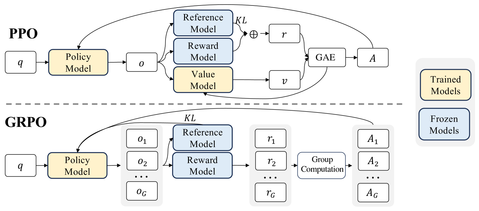
Comparison between PPO and GRPO architectures. Image from the DeepSeekMath paper [5].

1. Value Network vs. Group-Based Advantage:
   • PPO: Uses a separate value network \(V(s_t)\) to compute a baseline via TD errors, stabilizing advantage estimates.
   • GRPO: Eliminates the value network, computing advantages by comparing multiple outputs for the same prompt and normalizing via group statistics.

2. Reward Assignment:
   In many LLM applications, rewards are sparse and typically assigned only to the final token or overall output. PPO’s token-level value estimation can struggle in this setting, whereas GRPO leverages group comparisons to compute a robust, relative advantage.

3. Explicit KL Divergence Penalty:
   • PPO: Uses a clipping mechanism to limit policy updates.
   • GRPO: In addition to clipping, it includes an explicit KL divergence penalty
   \[-\beta\,D_{\mathrm{KL}}\!\bigl[\pi_\theta \,\|\, \pi_{\mathrm{ref}}\bigr],\]

   which directly penalizes deviations from a reference policy.

4. Stability Considerations:
   The group-based normalization and KL penalty in GRPO work together to maintain stable policy updates, compensating for the absence of a traditional value network.

Summary

The introduction of training on high quality labelled data at scale using PPO by OpenAI was the first step in developing the LLMs that we use today. Despite the usefulness of PPO, having to train both the policy and the value network is expensive, both in terms of compute time and ram usage. DeepSeek’s introduction of GRPO marks an important step towards the next chapter. By removing the value network while showing no noticeable drop in performance, GRPO is an algorithmic innovation that allows LLMs to train with less compute and in turn costs. They have also opensourced these models trained on GRPO in the form of DeepSeek V3 and R1. This will hopefully further accelerate and democratise the adoption of AI going forward.

References

1. Sutton, R. S., & Barto, A. G. (2018). Reinforcement Learning: An Introduction. MIT Press. Link

2. OpenAI. (2019). Better Language Models and Their Implications. Link

3. OpenAI. (2021). OpenAI Codex. Link

4. Ouyang, L., Wu, J., Jiang, X., et al. (2022). Training language models to follow instructions with human feedback. arXiv preprint arXiv:2203.02155. Link

5. Shao, Z., Wang, P., Zhu, Q., Xu, R., Song, J., Zhang, M., Li, Y., Wu, Y., & Guo, D. (2024). DeepSeekMath: Pushing the Limits of Mathematical Reasoning in Open Language Models. arXiv preprint arXiv:2402.03300. Link