Reference Frames for Orbital Mechanics
In a classic two-body problem where two bodies have finite mass, their trajectories in space follow an elliptical orbit. When the mass of one body is much larger than that of the other, \(m_1 \gg m_2\), we can approximate the larger body as stationary while the smaller body orbits around it. The trajectory of the smaller body can be modeled with either the Keplerian or Cartesian reference frames, each with its own pros and cons. The Cartesian reference frame is more useful for numerical calculations, such as computing future trajectories given the current state of the object. The Keplerian frame on the other hand provides a more intuitive understanding of the orbit by describing its phase space in mathematical terms.
Cartesian Reference Frame
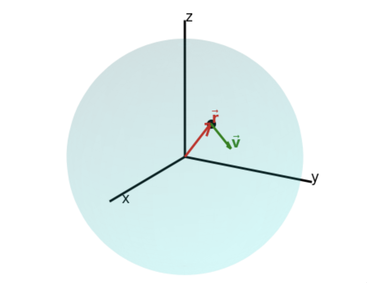
This is the reference frame that most people are familiar with, defined by the position \(\vec{r} = [x, y, z]\) and velocity \(\vec{v} = [v_x, v_y, v_z]\) of an object. It is an inertial reference frame with the more massive body(typically Earth) at its point of reference. The Cartesian state vector is a six-dimensional vector formed by concatenating the position and velocity vectors:
\[\vec{c} = [x, y, z, v_x, v_y, v_z].\]Together with the gravitational parameter \(\mu\), this state vector is sufficient to calculate the future trajectory of the object.
Keplerian Reference Frame
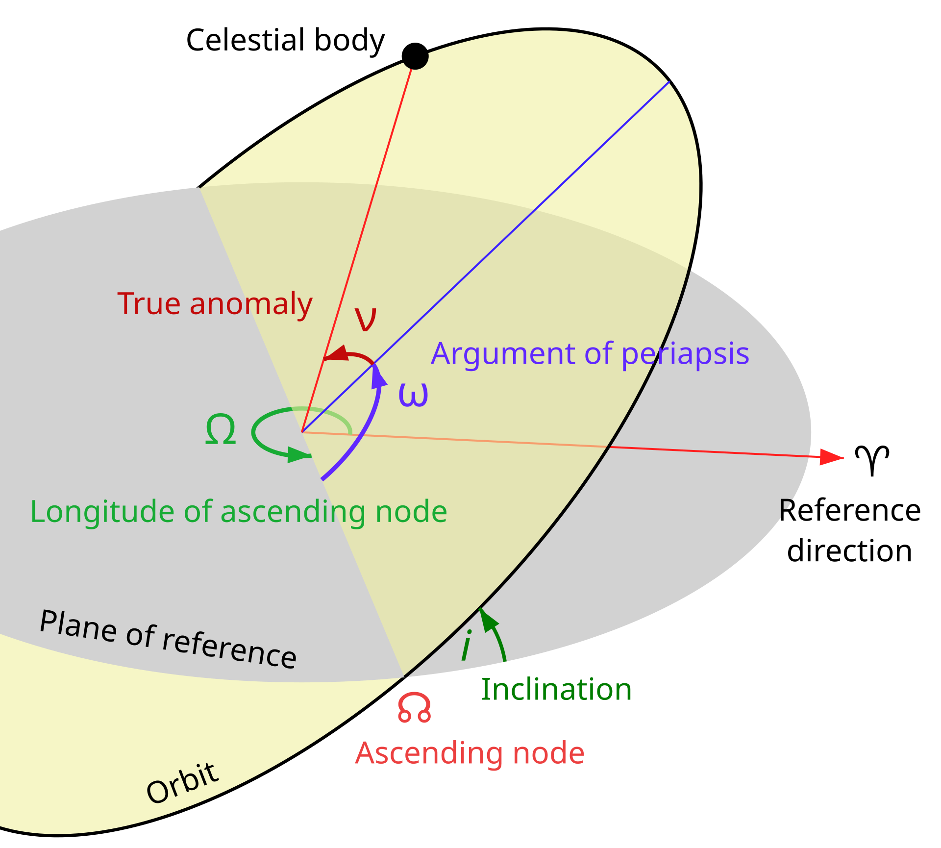
Image from Wikipedia.
In the Keplerian reference frame, an orbit is described not by instantaneous position and velocity components but by six orbital elements that capture the shape, size, orientation, and current position along the orbit. These six elements are:
-
Semimajor Axis, \(a\)
Defines the size of the orbit–the average distance between the orbiting object and the central body. -
Eccentricity, \(e\)
Describes the shape of the orbit. An eccentricity of 0 corresponds to a circular orbit, while values between 0 and 1 indicate an elliptical orbit. -
Inclination, \(i\)
Represents the tilt of the orbital plane relative to a chosen reference plane (often the equatorial or ecliptic plane). -
Right Ascension of the Ascending Node, \(\Omega\)
The angle in the reference plane from a fixed direction (typically the vernal equinox) to the point where the orbiting body crosses the reference plane upward (the ascending node). -
Argument of Periapsis, \(\omega\)
Measured in the orbital plane, this angle specifies the direction of the closest approach (periapsis) relative to the ascending node. -
True Anomaly, \(\nu\)
Indicates the object’s current position along its orbit relative to the periapsis, measured in the orbital plane.
These elements combine to form the Keplerian state vector:
\[\vec{k} = [\,a,\; e,\; i,\; \Omega,\; \omega,\; \nu\,].\]Together with the gravitational parameter \(\mu\), this six-element vector fully defines the orbit in the two-body problem. Although it does not directly include position and velocity components, these orbital elements encapsulate all the necessary information–through Kepler’s laws and the laws of motion–to compute the object’s future trajectory.
Given \(\vec{k}\) and \(\mu\), one can derive the instantaneous Cartesian state vector (and vice versa) using established transformation formulas. This makes the Keplerian state vector not only a compact representation of the orbit’s geometry but also sufficient for predicting the motion of the orbiting object over time.
Derivation of the Conic Section Orbit Equation and Its Conversion to Cartesian Coordinates
In orbital mechanics, the motion of a secondary body under the gravitational influence of a primary (central) body is governed by an inverse-square force. The resulting trajectory is a conic section (ellipse, parabola, or hyperbola). In the bound case (negative total energy), the orbit is an ellipse, and its shape and orientation can be described by six Keplerian orbital elements:
\[\vec{k} = [\,a,\; e,\; i,\; \Omega,\; \omega,\; \nu\,],\]where:
- \(a\) is the semimajor axis (size of the orbit),
- \(e\) is the eccentricity (shape of the orbit),
- \(i\) is the inclination (tilt of the orbital plane),
- \(\Omega\) is the right ascension of the ascending node (orientation of the line of nodes in the reference plane),
- \(\omega\) is the argument of periapsis (angle from the ascending node to periapsis within the orbital plane),
- \(\nu\) is the true anomaly (the current position along the orbit measured from periapsis).
Together with the gravitational parameter \(\mu\), these elements fully define the orbit in a two-body problem. We now describe, step by step, how the conic orbit equation is derived and how the Keplerian state vector is converted into the Cartesian (inertial) state vector.
1. Derivation of the Conic Section Orbit Equation
a. Newton’s Equation of Motion
For a body moving under the gravitational force of a central mass, Newton’s law gives:
\[\ddot{\mathbf{r}} = -\frac{\mu}{r^3}\mathbf{r},\]where \(\mu = G(M+m)\) (often approximated as \(GM\) when \(M \gg m\)). In polar coordinates (with variables \(r\) and \(\theta\)), the position vector is
\[\mathbf{r} = r\,\hat{\mathbf{r}}.\]b. Conservation of Angular Momentum
Angular momentum per unit mass, \(h\), is conserved:
\[h = |\mathbf{r} \times \dot{\mathbf{r}}| = r^2 \dot{\theta} = \text{constant}.\]This implies the rate of change of the angle is:
\[\dot{\theta} = \frac{h}{r^2}.\]c. Substituting \(u = \frac{1}{r}\)
To solve for the shape of the orbit \(r(\theta)\), it’s convenient to use the reciprocal variable:
\[u(\theta) = \frac{1}{r}.\]We need to relate time derivatives to derivatives with respect to \(\theta\). Using the chain rule and the conservation of angular momentum:
\[\dot{r} = \frac{dr}{d\theta}\dot{\theta} = \frac{dr}{d\theta} \frac{h}{r^2} = -h \frac{du}{d\theta}.\]Similarly, the second time derivative is:
\[\ddot{r} = \frac{d}{dt}\left(-h \frac{du}{d\theta}\right) = -h \frac{d^2u}{d\theta^2} \dot{\theta} = -h \frac{d^2u}{d\theta^2} \frac{h}{r^2} = -h^2 u^2 \frac{d^2u}{d\theta^2}.\]Substituting \(\ddot{r}\) and \(r\dot{\theta}^2 = r(h/r^2)^2 = h^2/r^3 = h^2 u^3\) into the radial component of Newton’s equation of motion (\(\ddot{r} - r\dot{\theta}^2 = -\mu/r^2\)) gives:
\[-h^2 u^2 \frac{d^2u}{d\theta^2} - h^2 u^3 = -\mu u^2.\]Dividing by \(-h^2 u^2\) yields the differential equation:
\[\frac{d^2 u}{d\theta^2} + u = \frac{\mu}{h^2}.\]d. Solving the Differential Equation
This is a linear second-order non-homogeneous differential equation with constant coefficients. Its general solution is the sum of the homogeneous solution (\(A\cos(\theta - \theta_0)\)) and a particular solution (\(\mu/h^2\)):
\[u(\theta) = A\cos(\theta - \theta_0) + \frac{\mu}{h^2},\]where \(A\) and \(\theta_0\) are constants determined by the initial conditions. We can choose the coordinate system such that \(\theta_0 = 0\) (meaning \(\theta=0\) corresponds to the point of closest approach, periapsis). Then, defining the eccentricity \(e\) via the constant \(A\):
\[e = \frac{A h^2}{\mu},\]we can write the solution as:
\[u(\theta) = \frac{\mu}{h^2}\left(1 + e\cos\theta\right).\]Since \(u = 1/r\), the orbit equation becomes:
\[\frac{1}{r} = \frac{\mu}{h^2}\left(1 + e\cos\theta\right).\]Rearranging gives the distance \(r\) as a function of the angle \(\theta\) (which is the true anomaly, commonly denoted by \(\nu\), so we replace \(\theta\) with \(\nu\)):
\[r(\nu) = \frac{h^2/\mu}{1 + e\cos\nu}.\]Defining the semi-latus rectum as \(p = h^2/\mu\), the polar equation of the orbit is:
\[\boxed{r(\nu) = \frac{p}{1 + e\cos\nu}.}\]Relationship between \(p\) and \(a\) for an ellipse: For an elliptical orbit (\(0 \le e < 1\)), the semi-latus rectum \(p\) is related to the semimajor axis \(a\) by \(p = a(1-e^2)\). Therefore, the orbit equation can also be written as:
\[r(\nu) = \frac{a(1-e^2)}{1 + e\cos\nu}.\]Interpretation:
- For \(e = 0\), the orbit is circular (\(r = a\)).
- For \(0 < e < 1\), the orbit is elliptical.
- For \(e = 1\), the orbit is parabolic (\(p\) is finite, but \(a\) is infinite).
- For \(e > 1\), the orbit is hyperbolic (\(a\) is negative by convention, \(p = a(1-e^2)\) is still positive).
2. Converting the Keplerian Elements to a Cartesian State Vector
Now that we have the orbit’s shape (\(r\) as a function of \(\nu\)), we derive the Cartesian position and velocity vectors in the inertial frame.
a. Position in the Perifocal (PQW) Frame
We first find the position vector in the orbital plane frame, often called the perifocal or PQW frame. In this frame:
- The P-axis (\(\hat{\mathbf{P}}\)) points from the central body towards the periapsis.
- The Q-axis (\(\hat{\mathbf{Q}}\)) is rotated 90 degrees from P in the direction of motion.
- The W-axis (\(\hat{\mathbf{W}}\)) is perpendicular to the orbital plane, such that \(\hat{\mathbf{W}} = \hat{\mathbf{P}} \times \hat{\mathbf{Q}}\), forming a right-handed system.
with
\[r = \frac{a(1-e^2)}{1 + e\cos\nu}.\]Substitute to obtain:
\[\mathbf{r}_{PQW} = \begin{bmatrix} \displaystyle \frac{a(1-e^2)\cos\nu}{1 + e\cos\nu} \\[1mm] \displaystyle \frac{a(1-e^2)\sin\nu}{1 + e\cos\nu} \\[1mm] 0 \end{bmatrix}.\]b. Velocity in the Perifocal (PQW) Frame
The velocity in polar coordinates has a radial component \(v_r = \dot{r}\) and a transverse component \(v_\theta = r\,\dot{\nu}\).
From conservation of angular momentum, we have:
\[h = \sqrt{\mu\,a(1-e^2)} \quad \text{and} \quad \dot{\nu} = \frac{h}{r^2}.\]Differentiate the orbit equation with respect to \(\nu\):
\[\frac{dr}{d\nu} = \frac{a(1-e^2)e\sin\nu}{(1+e\cos\nu)^2}.\]Then, applying the chain rule:
\[v_r = \dot{r} = \frac{dr}{d\nu}\,\dot{\nu} = \frac{a(1-e^2)e\sin\nu}{(1+e\cos\nu)^2} \cdot \frac{h}{r^2}.\]Since
\[r^2 = \frac{a^2(1-e^2)^2}{(1+e\cos\nu)^2},\]we simplify to:
\[v_r = \frac{h\,e\sin\nu}{a(1-e^2)}.\]The transverse component is:
\[v_\theta = r\,\dot{\nu} = \frac{h}{r} = \frac{h\,(1+e\cos\nu)}{a(1-e^2)}.\]The velocity vector in the PQW frame is then given by:
\[\mathbf{v}_{PQW} = \begin{bmatrix} v_r\cos\nu - v_\theta\sin\nu \\[1mm] v_r\sin\nu + v_\theta\cos\nu \\[1mm] 0 \end{bmatrix}.\]After substituting the expressions for \(v_r\) and \(v_\theta\) and simplifying, we obtain the commonly used form:
\[\mathbf{v}_{PQW} = \begin{bmatrix} -\sqrt{\dfrac{\mu}{p}}\,\sin\nu \\[1mm] \sqrt{\dfrac{\mu}{p}}\,(e+\cos\nu) \\[1mm] 0 \end{bmatrix},\]with \(p = a(1-e^2)\).
c. Transforming from the Perifocal Frame to the Inertial (Cartesian) Frame
To obtain the Cartesian state vector in an inertial frame (often Earth-Centered Inertial), we perform three successive rotations:
- Rotate by \(-\omega\) about the z-axis.
- Rotate by \(-i\) about the x-axis.
- Rotate by \(-\Omega\) about the z-axis.
The combined rotation matrix is given by:
\[Q_{Xx} = R_z(-\Omega)\, R_x(-i)\, R_z(-\omega),\]or equivalently (depending on the chosen convention):
\[Q_{Xx} = \begin{bmatrix} \cos\Omega\cos\omega - \sin\Omega\sin\omega\cos i & -\cos\Omega\sin\omega - \sin\Omega\cos\omega\cos i & \sin\Omega\sin i \\ \sin\Omega\cos\omega + \cos\Omega\sin\omega\cos i & -\sin\Omega\sin\omega + \cos\Omega\cos\omega\cos i & -\cos\Omega\sin i \\ \sin\omega\sin i & \cos\omega\sin i & \cos i \end{bmatrix}.\]Thus, the Cartesian position and velocity vectors are:
\[\mathbf{r}_{ECI} = Q_{Xx}\,\mathbf{r}_{PQW},\] \[\mathbf{v}_{ECI} = Q_{Xx}\,\mathbf{v}_{PQW}.\]Summary
-
Conic Section Orbit Equation:
\[r(\theta) = \frac{p}{1 + e\cos\theta}, \quad \text{with } p = \frac{h^2}{\mu}.\] -
Perifocal (PQW) Position:
\[\mathbf{r}_{PQW} = \begin{bmatrix} \displaystyle \frac{a(1-e^2)\cos\nu}{1 + e\cos\nu} \\[1mm] \displaystyle \frac{a(1-e^2)\sin\nu}{1 + e\cos\nu} \\[1mm] 0 \end{bmatrix}.\] -
Perifocal (PQW) Velocity:
\[\mathbf{v}_{PQW} = \begin{bmatrix} -\sqrt{\dfrac{\mu}{p}}\,\sin\nu \\[1mm] \sqrt{\dfrac{\mu}{p}}\,(e+\cos\nu) \\[1mm] 0 \end{bmatrix}.\] -
Transformation to the Inertial Frame:
\[\mathbf{r}_{ECI} = Q_{Xx}\,\mathbf{r}_{PQW},\quad \mathbf{v}_{ECI} = Q_{Xx}\,\mathbf{v}_{PQW},\]where the rotation matrix \(Q_{Xx}\) incorporates rotations by \(-\omega\), \(-i\), and \(-\Omega\).
This complete derivation demonstrates how the Keplerian elements define a conic (elliptical) orbit and how to mathematically convert that description into the Cartesian state vector needed for numerical trajectory prediction.